BECKMANN WORLD MODELS 01 · RESEARCH NOTES
Building a one-step
world model
From Beckmann transport to action-conditioned video: the objective, the failed trials, and what improved.
A world model is useful when it can answer a practical question: given what I have seen, what happens if I take these actions? If we want to compare many candidate actions, the cost of imagining each future matters.
Our starting point is a direct endpoint map: noise, recent observations, and actions go in; a future video chunk comes out in one network call. This post explains how we adapted Beckmann Transport Models to that setting—and why the transport objective alone was only the beginning.
PushT
SPATIAL EPOCH 30Robomimic Can
SPATIAL EPOCH 30In this article
- From denoising to direct maps
- The endpoint-map idea
- Making the map a world model
- Trials that changed the recipe
- What 30 spatial epochs changed
- Looking beyond the averages
- What one step buys
- Prediction is not planning
- Bridge-V2 and RT-1 in latent space
- What we would carry forward
- References & experiment record
01From denoising to direct maps
Diffusion models learn to reverse a noise-corruption process. Sampling follows a sequence of model evaluations from noise toward data. A world model repeats this process whenever it needs another future chunk, multiplying the cost across time and candidate action sequences.
Faster samplers and consistency models shorten this path. Consistency training can be standalone or distilled; a pretrained teacher is not a requirement of every few-step approach. The broader question is whether we can train a useful one-call generator directly.
Drifting models take that route by evolving the generated distribution during training, using attraction toward data and repulsion among generated samples. DriftWorld brings this idea to action-conditioned video. It is an important one-step comparison: our speed advantage is over iterative diffusion, not over other one-call models.
Beckmann transport gives us a different organizing principle: learn the destination associated with an autonomous trajectory. We use that principle to train a conditional map, then add supervision aimed at the endpoint a world model actually produces.
02The endpoint-map idea
Fix the context , where is the observed history and is a proposed action sequence. For an autonomous flow, the terminal map is constant along a trajectory. Its differential form and data boundary condition are:
For RGB video, our map is a residual U-Net. It receives the future tensor being transported, four history frames, and action embeddings. The inference rule is simply:
One call predicts four future frames on PushT or two on Robomimic Can, at 96 × 96 resolution. We append the prediction to the history and repeat. The network has no interpolation-time input; this is a time-independent endpoint map.


What the training update actually computes
We sample a straight interpolation between Gaussian source and recorded future . A Jacobian–vector product (JVP) measures how the endpoint map changes along the source-to-target chord, holding history and actions fixed:
means stop-gradient. The target is detached, so optimization regresses the map toward a stopped update; it does not backpropagate through a squared JVP using second derivatives. The chord is a sampling device, not the actual autonomous characteristic, and individual sampled JVPs need not be zero.
The last two terms anchor the data boundary and the neighborhood near data. Squared norms here use coordinate means; the near-data term is averaged over the whole batch. A detached coefficient balances transport and anchor gradient norms on the last spatial output layer. Implementation ↗
A training-step sketch
# h and a stay fixed inside the forward-mode JVP.
x = (1 - s) * z + s * y
p, q = jvp(lambda x: T(x, h, a), x, y - z)
target = stop_gradient(p + 0.25 * q)
transport = normalized_residual(p, target)

# Supervise the exact query used at deployment.
prediction = T(z, h, a)
loss = balanced_transport_and_anchors(transport)
loss += source_loss(prediction, y)
loss += motion_temporal_range_losses(prediction, y)
loss += spatial_feature_loss(prediction, y)
# Short detached-history recovery runs on scheduled updates.
Conceptual pseudocode. Ramps, weighting, and recovery scheduling are described below; the linked research code is authoritative.
03Making the map a world model
Transport geometry describes a map over the future tensor. World modeling adds two demands: the prediction must correspond to the supplied actions, and the model must remain useful when its history contains earlier predictions. We addressed these through the training recipe.
1. Put supervision on the pure-noise query
A correct boundary value does not directly supervise , the query used at inference. Source loss does. Its coefficient ramps to one over 500 updates, outside the transport-loss balancing rule.
There is a tradeoff: squared error rewards the conditional mean and penalizes variation across source draws. At fixed context and target, the error decomposes into mean error plus sampling variance:
Lower error therefore does not prove that a generator preserves all plausible futures. Conditional diversity remains an open evaluation question.
2. Emphasize motion and tolerate imperfect history
Most pixels in a manipulation scene can stay almost unchanged. We add a target-motion-weighted loss, a within-chunk temporal-difference loss, and a penalty for predictions outside the normalized RGB range:
The moving-region denominator has a floor so sparse motion does not amplify the loss excessively. Every fourth update also uses short generated-history recovery: earlier predictions are detached, and only the last prediction receives gradients. Its weight ramps to 0.25 over 1,000 updates.
The recorded future remains the training target, so this is a local robustness regularizer, not supervision for arbitrary counterfactual histories. We retain unclipped RGB feedback during evaluation. The working continuation also uses a quarter of the earlier learning rate; the observed gains belong to the complete recipe.
3. Compare spatial features at the output
Pixel error alone gives a limited description of object structure. We add a loss between spatial VGG16 feature maps of the source prediction and target, using relu1_2, relu2_2, and relu3_3:
Features are normalized across channels at each location, then channel-squared differences are summed and averaged across locations, frames, and examples. The feature extractor is frozen, but gradients flow through its input into the prediction. The weight ramps to 0.05 over 1,000 updates.
This is output supervision using pretrained features; it is not the learned LPIPS evaluation metric. VGG is absent at inference. The RGB generator is trained without a pretrained generative teacher.
PushT
Robomimic Can
04Trials that changed the recipe
The most useful experiments were not all wins. Two branches tested whether adding a learned transport direction or propagating gradients through connected predictions would improve the existing map.
A learned direction did not transfer reliably
We added a head to predict the chord direction and gradually substituted it into the JVP. On Can, 64-frame MSE rose from 0.0068 to 0.0203 and LPIPS from 0.0225 to 0.0854. PushT improved in this continuation, so the evidence argues against adopting it as a reliable default—not against every learned-direction method.
The Can map was already deteriorating before the learned tangent was enabled. The auxiliary head shared decoder features and a clipping group with the endpoint model. That makes auxiliary-task interference a plausible explanation; the logs do not establish its share of the damage or rule out optimizer-restart effects. [audit]
More connected gradients were not automatically better
The attached variant backpropagated through two connected predictions at the full learning rate. The detached recovery recipe used a lower learning rate and performed better on the final 64-frame metrics for both tasks. Because both the gradient path and optimization recipe changed, this comparison does not isolate detachment alone.
| Training recipe | PushT MSE ↓ | PushT LPIPS ↓ | PushT full ↓ | Can MSE ↓ | Can LPIPS ↓ | Can full ↓ |
|---|---|---|---|---|---|---|
| Source-supervised map | 0.0293 | 0.0746 | 0.0434 | 0.0068 | 0.0225 | 0.0940 |
| + learned direction | 0.0208 | 0.0501 | 0.0319 | 0.0203 | 0.0854 | 0.0759 |
| Robust · detached / lower LR | 0.0199 | 0.0564 | 0.0299 | 0.0031 | 0.0090 | 0.0112 |
| Robust · attached / full LR | 0.0225 | 0.0808 | 0.0338 | 0.0051 | 0.0215 | 0.0146 |
Table 1. Completed trial endpoints, rounded as recorded. Full = full-episode autoregressive MSE. Direction continues from the source checkpoint; robust variants branch from that source parent. These are single training runs with different cumulative budgets. Source logs ↗
Can also exposed a gap between short and long rollouts. The source model’s 64-frame MSE was 0.0068, but full-episode MSE was 0.0940, with a worst-episode value of 0.737. The robust recipe reduced full-episode MSE to 0.0112. Good short-window prediction had not been enough to make repeated feedback reliable.
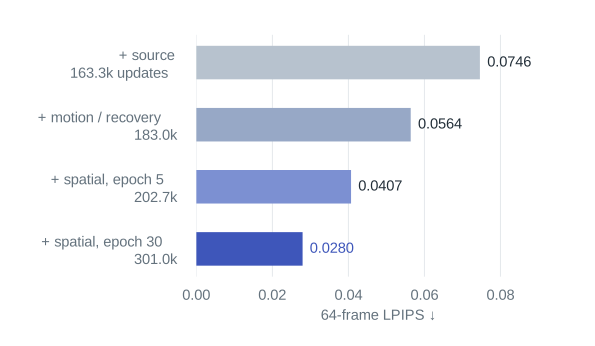
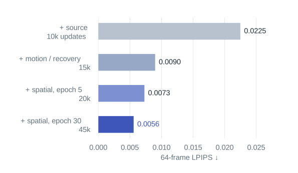
Spatial supervision subsequently improved 64-frame quality, but not every number moved together: Can’s full-episode MSE was 0.0112 for the robust model and 0.0114 after five spatial epochs. We kept the full-episode measurements visible while extending training.
05What 30 spatial epochs changed
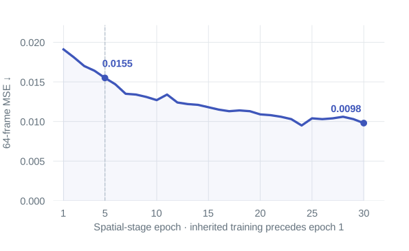
The completed spatial continuations produce the strongest final RGB prediction metrics in our local comparison. Relative to spatial epoch five, 64-frame MSE falls from 0.0155 to 0.0098 on PushT and from 0.0028 to 0.0022 on Can. The improvements require no additional inference steps.
PushT
Robomimic Can
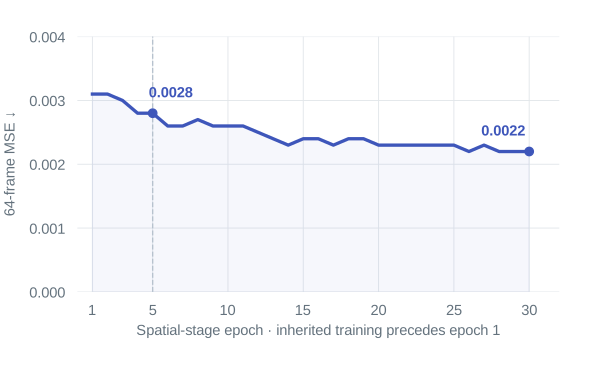
“30 epochs” refers to the spatial stage, not the model’s whole training history. Including inherited training, the final models use 301,028 updates on PushT and 45,000 on Can. Update counts also do not equal compute: batch sizes and per-update costs can differ.
64 frames = 4 observed + 60 generated; RGB is normalized to [−1, 1]. PushT uses 388 eligible 64-frame videos and 400 full episodes; Can uses 30 for both. “Moving MSE” emphasizes the moving region. Lower is better except SSIM. Local baseline runs use five epochs; BWM rows include inherited training.
| Model / checkpoint | Calls / chunk | MSE ↓ | Moving MSE ↓ | LPIPS ↓ | SSIM ↑ | Full MSE ↓ |
|---|---|---|---|---|---|---|
| BWM + spatialspatial epoch 30 · final | 1 | 0.0098 | 0.1247 | 0.0280 | 0.975 | 0.0154 |
| BWM + spatialspatial epoch 5 | 1 | 0.0155 | 0.1933 | 0.0407 | 0.964 | 0.0231 |
| BWMrobust recipe | 1 | 0.0199 | 0.2419 | 0.0564 | 0.953 | 0.0299 |
| DriftWorld5-epoch baseline | 1 | 0.0314 | 0.4093 | 0.0790 | 0.927 | 0.0451 |
| MSE U-Net5-epoch baseline | 1 | 0.0303 | 0.4008 | 0.0804 | 0.943 | 0.0427 |
| GPC diffusion5-epoch baseline | 12 | 0.0630 | 1.4241 | 0.1609 | 0.904 | 0.0753 |
| AVDC diffusion5-epoch baseline | 100 | 0.0684 | 1.1840 | 0.1860 | 0.895 | 0.0795 |
Table 2. PushT, held-out rollout evaluation. Calls are per four-frame future chunk.
| Model / checkpoint | Calls / chunk | MSE ↓ | Moving MSE ↓ | LPIPS ↓ | SSIM ↑ | Full MSE ↓ |
|---|---|---|---|---|---|---|
| BWM + spatialspatial epoch 30 · final | 1 | 0.0022 | 0.0242 | 0.0056 | 0.984 | 0.0082 |
| BWM + spatialspatial epoch 5 | 1 | 0.0028 | 0.0298 | 0.0073 | 0.979 | 0.0114 |
| BWMrobust recipe | 1 | 0.0031 | 0.0316 | 0.0090 | 0.974 | 0.0112 |
| DriftWorld5-epoch baseline | 1 | 0.0104 | 0.0769 | 0.0682 | 0.856 | 0.0256 |
| MSE U-Net5-epoch baseline | 1 | 0.0051 | 0.0544 | 0.0104 | 0.969 | 0.0138 |
| GPC diffusion5-epoch baseline | 6 | 0.0276 | 0.3103 | 0.0589 | 0.910 | 0.0380 |
| AVDC diffusion5-epoch baseline | 100 | 0.0400 | 0.2644 | 0.1194 | 0.801 | 0.1768 |
Table 3. Robomimic Can, held-out rollout evaluation. Calls are per two-frame future chunk. Tables 2–3 compare deployed checkpoints, not equal total training compute. Evaluation sources ↗
For context, a released long-trained DriftWorld checkpoint on PushT records MSE 0.0085 and LPIPS 0.0163 after about 1.18 million updates—better than our final values. Its exclusion of these evaluation episodes is unverified, so we show it as a reference rather than a controlled ranking. The evidence supports an improving one-step recipe, not a universal state-of-the-art claim.
06Looking beyond the averages
Averages hide where a model loses the scene. The viewer below synchronizes all methods on the same saved episode. It comes from the earlier spatial-epoch-five comparison; Figure 1 contains the new epoch-30 predictions.
Video could not load. Please select another example.
Even at epoch 30, some PushT predictions become visibly blurred or diverge from the recorded block configuration later in the rollout. The examples below make those remaining errors easy to inspect. We cannot attribute their cause from appearance alone.
PushT · example 06
PushT · example 08
07What one step buys
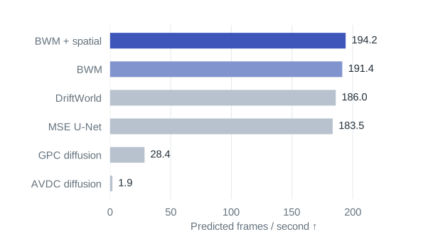
On a dedicated A800, the spatial-epoch-five RGB model takes 20.6 ms per PushT chunk and 23.9 ms per Can chunk. Accounting for four versus two output frames gives 193.9 and 83.8 predicted frames per second, respectively.
PushT · four frames / call
Can · two frames / call
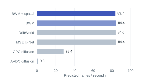
The measured gains are approximately 6.8× / 2.9× over GPC and 101× / 99× over AVDC for PushT / Can. DriftWorld and the regression U-Net are already one-call models with similar latency. For those comparisons, the question is prediction quality and training behavior, not fewer sampling steps. [timings]
08Prediction is not planning
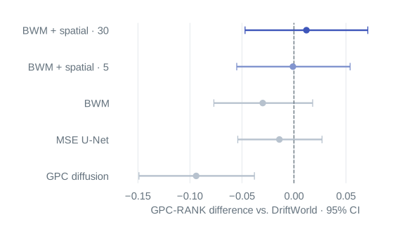
PushT planning uses a frozen pose reader to score the last predicted frame for candidate action sequences. The planner needs to order nearby alternatives correctly. That is a different requirement from reducing average error along recorded trajectories.
The final BWM model scores 0.721 on GPC-RANK, versus 0.709 for the local DriftWorld baseline. The paired difference is +0.012 with a 95% interval of [−0.047, +0.071]. This does not establish a planning improvement.
| Model | Planning ↑ | Policy r ↑ | IoU MAE ↓ |
|---|---|---|---|
| BWM + spatialspatial epoch 30 | 0.721 | 0.928 | 0.010 |
| BWM + spatialspatial epoch 5 | 0.708 | 0.946 | 0.010 |
| DriftWorld5-epoch baseline | 0.709 | 0.857 | 0.031 |
| MSE U-Net5-epoch baseline | 0.695 | 0.915 | 0.012 |
| GPC diffusion5-epoch baseline | 0.615 | 0.366 | 0.513 |
Table 4. Planning and policy-outcome prediction. Policy estimates use seven policies × 300 paired trials. MAE is the absolute error in predicted policy IoU; it is not a robot success rate. Values are rounded. Evaluation record ↗
Do the actions actually matter?
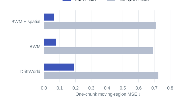
In a 64-window probe, swapping actions while holding real history fixed increases the spatial model’s moving-region error by 11.0× on PushT and 6.2× on Can. The predictions respond to the action input, rather than relying only on visual history.
PushT
Robomimic Can
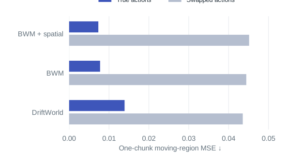
A useful next target is candidate-ranking error: whether the model prefers the action that really produces the better outcome. Neither a sharp frame nor a large action-swap penalty answers that question on its own.
09Bridge-V2 and RT-1 in latent space
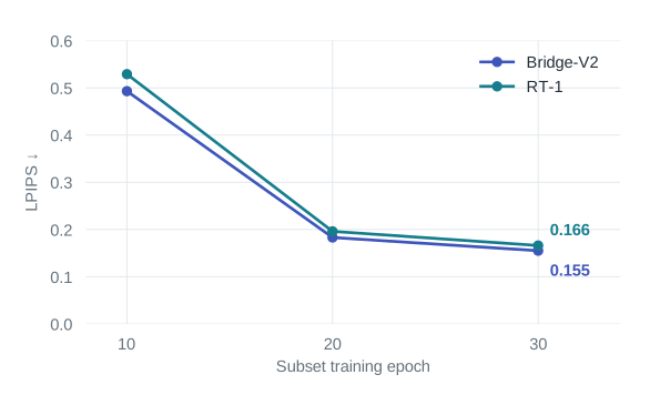
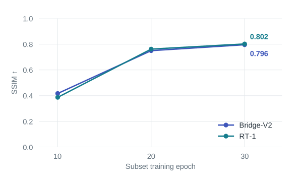
We also transferred the recipe to 256-pixel robot video. The native model uses SD3 VAE latents with 16 channels at 32 × 32 resolution and a DriftWorld-style native U-Net: 175.4M parameters for Bridge-V2 and 160.3M for RT-1.
Each call predicts one latent frame, conditioned on four context frames and actions. The spatial and range losses operate through the decoded endpoint; the temporal term is zero for a one-frame output. The pretrained VAE remains part of this system.
The completed subset runs use 2,078 eligible training episodes on Bridge and 2,041 on RT-1. Unlike the RGB continuations, these runs schedule map, source, robustness, and spatial stages within a single 30-epoch subset budget.
Perceptual error
Structural similarity
| Dataset | SSIM ↑ | PSNR ↑ | LPIPS ↓ | FID ↓ | FVD ↓ | Calls / frame |
|---|---|---|---|---|---|---|
| Bridge-V2 | 0.796 | 22.13 | 0.155 | 68.86 | 592.24 | 1 |
| RT-1 | 0.802 | 23.15 | 0.166 | 75.53 | 535.59 | 1 |
Table 5. Final epoch-30 subset results. Bridge: 215 validation videos / 7,079 predicted frames. RT-1: 198 / 8,409. FVD uses 201 / 193 eligible videos and their first 16 generated frames.
Generator time is 16.3 ms per Bridge frame and 13.1 ms per RT-1 frame; VAE decoding adds about 26 ms per frame. The latest run table also records approximately 2.8 and 2.3 training GPU-hours for the subset runs, excluding evaluation.
At the September 29, 04:16 UTC source snapshot, full-data continuations were still training and matched-subset baselines were queued. There are no completed full-data results to report. Snapshot ↗ · Latest run table ↗
10What we would carry forward
The practical contribution is a direct conditional map whose output is supervised where it is used: at the Gaussian source, under imperfect history, and in spatial feature space. The strongest evidence is the completed improvement in video prediction while retaining one-call generation.
- Keep the inference query central. A transport-inspired objective still needs to train the operation deployed in the world model.
- Audit the entire training lineage. An epoch label for the last stage is not a total training budget.
- Keep the unsuccessful trials. A learned direction and more connected gradients did not reliably beat the simpler working recipe.
- Evaluate the downstream decision separately. Planning, conditional diversity, and counterfactual accuracy remain distinct from image quality.
The immediate open questions are whether these gains persist in matched native comparisons, whether useful conditional variation survives source supervision, and whether better endpoint structure improves action selection. The current measurements leave all three questions open.
References & experiment record
The September 25 manuscript predates the new results. This article uses saved evaluations and the September 29, 04:16 UTC repository snapshot for the updated experiment record.
- Denoising Diffusion Probabilistic Models. Background on iterative denoising.
- Consistency Models. One- and few-step generation, including standalone training.
- Generative Modeling via Drifting. Direct one-step generative training.
- DriftWorld: Fast World Modeling through Drifting. The one-step world-model comparison and native interfaces.
- Beckmann Transport Models: From Autonomous Flows to One-Step Maps. Terminal-map geometry and stopped-target training; our work adapts this foundation to world modeling.
- Trial records: Can source / direction, PushT source / direction, robust and spatial continuations.
- Direct-map causal audit and mathematical corrections. Mechanism hypotheses, gradient paths, and limits of the probes.
- RGB results: exact final metrics and checkpoint hashes, earlier baseline snapshot, spatial training record, comparison-video provenance.
- Dedicated inference-latency measurements. Hardware, precision, and model-call accounting.
- Downstream evaluations: policy evaluation, epoch-30 planning and policy results.
- Native Bridge-V2 / RT-1 snapshot. Completed subset evaluations, timing, and pending comparisons.
Beckmann World Models
Adam Lee · Shobhit Agarwal · JP Suh